Tensor Contractions on AWS Trainium2#
Tensor contractions are a fundamental operation across computational science and machine learning. They appear in the simulation of quantum circuits, in many-body and coupled-cluster electronic-structure methods, and throughout deep learning.
This website presents our compiler, which optimizes tensor contractions and lowers them to high-performance kernels for AWS Trainium2.
Mapping tensor contractions onto systolic arrays#
Domain-specific accelerators such as AWS Trainium2 deliver far higher throughput and energy efficiency than general-purpose hardware. Most of their computational power is in systolic arrays, specialized compute units that perform matrix multiplication in hardware. Each core of Trainium2 contains one such array with a 128x128 grid of processing elements. The array performs a matrix multiplication by holding one input stationary. One axis of that input is laid out along the 128 rows, a second axis along the 128 columns, and every processing element stores one element. The other input then streams through the array. The grid is therefore fully utilized only if both chosen axes have 128 elements. This design makes the accelerators efficient mainly on large and regular matrix-matrix multiplications.
Tensor contractions generalize matrix multiplication to higher dimensions, so
they are natural candidates for the same hardware. Mapping them onto the
array, however, remains challenging. Take the contraction
eafd,fbec -> abcd in einsum notation with
a=96, b=84, c=84, d=84, e=96, f=96, a case from the
Tensor Contraction Benchmark.
Every axis has at most 96 elements, so a direct mapping of an axis to the
array’s rows or columns leaves parts of them idle. For example, loading the
second input stationary with axis e along the rows and axis c along the
columns occupies 96x84 of the 128x128 processing
elements. This is a utilization of only 49%.
Four factors are critical to achieving high performance on Trainium2:
Maximize PE utilization. A single axis rarely matches the 128 elements of the array’s rows and columns. Splitting several axes and combining tiles can improve the utilization of the systolic array. For the contraction
eafd,fbec -> abcd, this can increase PE utilization to 98%.Minimize the overhead of data layout transformations. Mapping the operands onto the hardware requires data layout transformations. These can be performed during the loads and stores that move data between HBM and the chip, or by separate operations in on-chip memory. The placement determines which hardware resources the transformations occupy.
Overlap data movement with computation. Operands are kept in on-chip memory. Tiling determines how often each block loaded from HBM can be reused. Double buffering overlaps the data movements with computation.
Parallelize the contraction. On Trainium2, two NeuronCores share one HBM stack. They can be configured to work in parallel on the same data.
The Trainium2 architecture#
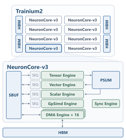
Fig. 1 Illustration of a Trainium2 device and one of its NeuronCores. Adapted from the AWS Neuron SDK documentation.#
Trainium2 is made up of eight NeuronCores-v3, with two NeuronCores sharing a single HBM stack (Fig. 1). Within a NeuronCore, four compute engines operate on data held in SBUF, the software-managed on-chip memory. The tensor engine performs matrix multiplications on its 128x128 systolic array and accumulates the results in PSUM, a dedicated partial-sum buffer. PSUM has only a limited capacity for partial results. We use the vector engine to add such partial results onto an accumulator held in SBUF. The scalar engine performs vector-scalar operations. Since it reads and writes a vector, we use it for data layout transformations. The GPSIMD engine is a general-purpose engine. It can be used to generate memory access descriptors for the DMA engines, which move data between off-chip HBM and SBUF. The Trainium2 Architecture Guide describes the architecture in further detail.
From tensor contractions to high-performance NKI kernels#
PE utilization, data layout transformations, and tiling are tightly coupled decisions. Combining several axes onto the tensor engine’s two dimensions increases PE utilization, but complicates the data transfers. Moving a layout transformation from the DMA engine onto other on-chip engines reduces this overhead, but takes extra SBUF memory for its intermediate results. The tiling, in turn, competes for the same SBUF memory to keep operand tiles available for reuse. The three choices must therefore be made together. Our compiler makes these coupled decisions automatically. It takes a tensor contraction, given as an einsum equation and its axis sizes, and compiles it into a kernel for the Neuron Kernel Interface (NKI).
1. Lower to TEIR. The contraction is lowered to an initial Tiled Execution Intermediate Representation (TEIR) graph, as shown in Fig. 2. It allocates the output tensor and wraps a 1x1x1 GEMM in a chain of loop nodes, one per axis of the contraction.
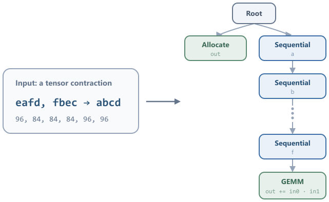
Fig. 2 The contraction eafd,fbec -> abcd and the corresponding, unoptimized TEIR
graph of scalar operations.#
2. Optimize TEIR. Fig. 3 shows our optimization pipeline, which rewrites the graph with three passes: normalize contraction, tiling search, and multicore parallelization. The normalization pass transforms the contraction into a normal form. It reorders chains of loop nodes and fuses loop nodes whose axes are adjacent in memory. The tiling search optimizes the contraction for a single core, and the multicore parallelization pass distributes the work across cores. Fig. 3 shows the tiling search in more detail. The search enumerates kernel tiling candidates crossed with SBUF tiling candidates. The kernel tiling selects the axes that are combined onto the tensor engine’s dimensions, and the number of elements each axis contributes. The SBUF tiling sets the number of elements per axis held in SBUF for reuse, and whether SBUF holds additional copies of a tensor for on-chip data layout transformations. Since the search space can become too large to score every candidate in reasonable time, we prune weak candidates directly. Retained kernel tilings must preserve the unit-stride axes of the tensors in the kernel. Retained SBUF tilings must maximize SBUF usage, forming a Pareto front. We keep the tilings where the number of elements of an axis cannot be increased without exceeding the capacity of SBUF. Only the survivors are realized into full schedules, with their memory allocations, data movements and tensor-engine operations, and scored by a measurement-based performance model. The model estimates the time of every operation on its engine (tensor, vector, scalar, and stride-aware DMA). It times the first iteration of a loop as if its operations ran sequentially. While one engine works, the others remain idle. This models the startup and cooldown costs that cannot be hidden. Each later iteration of the loop adds one steady-state period to the total time. Double buffering lets its operations slide into the idle times of neighboring iterations. The engine with the smallest idle time therefore decides how long that period is. This ranks candidates without running any of them on hardware.
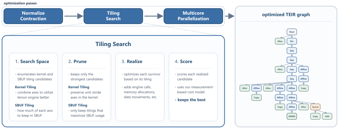
Fig. 3 The optimization passes, with the tiling search expanded below
them. On the right is the optimized TEIR graph for eafd,fbec -> abcd.#
3. Generate NKI code. A final walk over the optimized TEIR graph maps each node to the NKI constructs shown in Fig. 4 and emits the kernel.
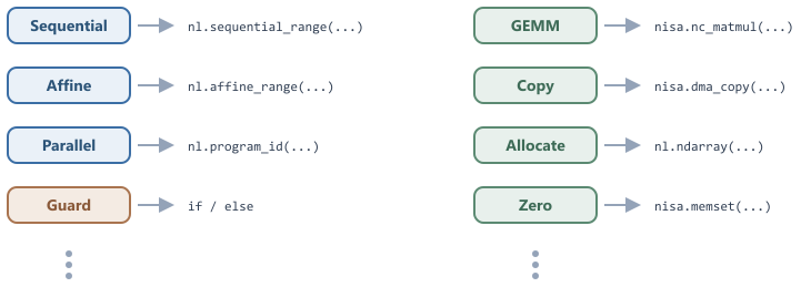
Fig. 4 Every TEIR node is lowered to NKI constructs.#
Evaluation#
We ran all measurements on a single AWS EC2 trn2.3xlarge instance with
one Trainium2 device, using two NeuronCores. The two cores share one HBM
stack and therefore operate on shared memory. Using more cores requires
communication between separate HBM stacks, which is outside the scope of this
work. The theoretical FP16 peak performance of the two cores is 157 TFLOPS.
Square matrix multiplication#
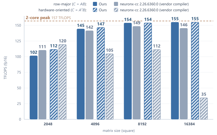
Fig. 5 Performance of square matrix multiplication with sizes of powers of two. We compare two data layouts for matrix A, effectively computing \(C = AB\) and \(C = A^{T}B\), against the vendor compiler neuronx-cc 2.26.6360.0. All measurements are in FP16 on two NeuronCores.#
Fig. 5 compares our kernels against the vendor compiler neuronx-cc for square matrix multiplication in two data layouts. The first is \(C = AB\) with all matrices stored row-major, the default layout of PyTorch tensors. The second is the hardware-oriented layout \(C = A^{T}B\). This aligns with the matrix multiplication the tensor engine computes, so the kernel needs no transpositions.
Our kernels reach up to 155 TFLOPS, 98.7% of the theoretical peak. For matrix multiplications of size 4096 and larger, the compiler outperforms neuronx-cc in both data layouts, by 2 to 6% for \(C = AB\) and by 1.4x to 4.4x for \(C = A^{T}B\). At 2048, neuronx-cc is ahead with 111 and 120 TFLOPS against our 102 and 112 for \(C = AB\) and \(C = A^{T}B\), respectively.
Tensor contractions#
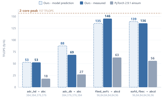
Fig. 6 Performance benchmarks of four cases from the Tensor Contraction Benchmark. Axis sizes are given in alphabetical index order. All measurements are in FP16 on two NeuronCores.#
We measured four contractions from the Tensor Contraction Benchmark, a collection of cases gathered from several publications. The four cases differ in memory layout and axis sizes.
Across all four contractions our compiler is 2.3x to 2.9x faster than
torch.einsum of PyTorch 2.9.1. On the two large contractions, fbed,aefc -> abcd and
eafd,fbec -> abcd, it reaches 146 and 136 TFLOPS. On the smaller
contractions, adc,bd -> abc and adc,db -> abc, our compiler only
achieves 53 and 69 TFLOPS. These contractions are too small to hide the
startup overheads. They also provide too little computation to fully overlap
the data movements.
The lighter bars in Fig. 6 show the predictions of our performance model
for the chosen schedule. On adc,bd -> abc and
eafd,fbec -> abcd the prediction comes within a few TFLOPS of the
measurement.
What comes next#
All measurements in this work used two NeuronCores that share one HBM stack, so the multicore parallelization pass can split a contraction without moving data between memories. Scaling further means partitioning a contraction across separate HBM stacks and eventually across devices. This requires explicit communication. A next step could extend the compiler to place these transfers and to weigh them in the performance model like any other data movement.