10. Tiled Execution IR

We have assembled the necessary tools to execute tensor operations efficiently. This chapter introduces the Tiled Execution Intermediate Representation (TEIR), which describes the execution of tensor operations through primitives that operate on subtensors, known as tiles. The IR guides the backend implementation and controls when and where primitives are executed. Conceptually, the IR is closely related to tile-based programming models such as Triton, CUDA Tile IR, Pallas, TileIR, and TileLang.

TEIR separates a tiled tensor operation into three components:

TEIR-Axes

Defines the available axes. An axis has an extent, per-tensor byte strides, and per-tensor byte offsets.

TEIR-Schedule

Defines a tree-shaped execution schedule. Iteration nodes iterate over axes; invocation nodes invoke primitives.

TEIR-Primitives

Defines the primitives that may be invoked from invocation nodes. A primitive declares the operation it performs and the axes it consumes internally.

The schedule decides when work is executed. The primitive component decides what work is executed at an invocation node. The axis component decides where each tile is located in memory. We call the component or tool that constructs a TEIR configuration the emitter.

10.1. TEIR-Axes

Table 10.1.1 Fields of a TEIR-Axes entry.

Field	Meaning	Domain and constraints
id	Unique axis identifier.	String or numeric identifier.
extent	Positive axis extent.	Positive integer.
strides	Per-tensor byte strides.	Array of non-negative integers, one per tensor. Zero stride means the tensor address does not depend on this axis.
offsets	Per-tensor byte offsets.	Array of integers, one per tensor. Offsets may be negative. Zero means no offset.

TEIR-Axes is a keyed collection of axis definitions. As shown in Table 10.1.1, each axis has a unique identifier. The stride vector contains one stride entry per tensor. The offset vector contains one offset entry per tensor. All strides and offsets are given in raw bytes. This makes the axis layout independent of the data type.

We discuss two examples in which the axes describe the dimensions and memory layout of two-dimensional tensors, i.e., matrices. For an axis identifier \(x\), we write \(|x|\) for its extent. In both examples, stride and offset tuples use tensor order \((T_0, T_1)\).

First consider two matrices \(T_0\) and \(T_1\) with the same logical axes \(a\) and \(b\). Matrix \(T_0\) stores FP32 elements and matrix \(T_1\) stores FP16 elements. Both have shape \(|a| \times |b| = 4 \times 8\).

Table 10.1.2 TEIR-Axes records for two matrices with the same logical axes.

Axis	Extent	Strides	Offsets	Interpretation
a	4	(32, 16)	(0, 0)	Row axis of both matrices.
b	8	(4, 2)	(0, 0)	Column axis of both matrices.

For row-major storage, the resulting axes are given in Table 10.1.2. The logical axes are identical, but the byte strides differ because the element sizes differ. For example, when advancing axis \(a\) we have to jump by \(|b|\) entries in both matrices: \(8 \cdot 4 = 32\) bytes in \(T_0\) and \(8 \cdot 2 = 16\) bytes in \(T_1\).

The second example keeps the same shared row axis \(a\) but gives the two matrices different column axes. Specifically, matrix \(T_0\) has shape \(|a| \times |b| = 4 \times 8\) with FP32 elements. Matrix \(T_1\) has shape \(|a| \times |c| = 4 \times 16\) with FP16 elements.

Table 10.1.3 TEIR-Axes records for two matrices with one shared axis.

Axis	Extent	Strides	Offsets	Interpretation
a	4	(32, 32)	(0, 0)	Shared row axis.
b	8	(4, 0)	(0, 0)	Column axis of \(T_0\).
c	16	(0, 2)	(0, 0)	Column axis of \(T_1\).

The resulting axes are shown in Table 10.1.3. Here the shared row axis \(a\) has the same byte stride in both matrices: \(8 \cdot 4 = 32\) bytes in \(T_0\) and \(16 \cdot 2 = 32\) bytes in \(T_1\). Axis \(b\) defines a zero stride for \(T_1\), while axis \(c\) defines a zero stride for \(T_0\). A zero stride means that varying this TEIR axis leaves the corresponding tensor address unchanged. More precisely, using a zero stride expresses the additive identity in the address calculation.

10.2. TEIR-Schedule

TEIR-Schedule is a forest of nodes that describes when each primitive is executed. A schedule consists of three pieces:

1. An ordered list roots of root node identifiers,

2. a collection of iteration nodes defined by Table 10.2.1,

3. and a collection of invocation nodes defined by Table 10.2.2.

Iteration nodes form the interior of the tree. Each one iterates one TEIR axis and owns an ordered list of children that may contain further iteration nodes or invocation nodes. Invocation nodes are the leaves of the tree, that is, each one invokes a primitive.

Every node has a unique identifier. The ID namespace is shared between iteration and invocation nodes. The sibling order is encoded explicitly by the list order of children. The top-level roots list provides the analogous order for the schedule’s root nodes. Because more than one root is allowed, the schedule is a forest in general.

An iteration node with policy = sequential traverses its axis in increasing index order. With policy = parallel the runtime or lowering decides the mapping and degree of parallelism.

Table 10.2.1 Fields of an iteration node.

Field	Meaning	Domain and constraints
id	Unique node identifier.	String or numeric identifier, unique across all schedule nodes.
axis	Iterated TEIR axis.	Identifier of an axis in TEIR-Axes.
policy	Iteration policy.	sequential or parallel.
children	Ordered list of child node identifiers.	Non-empty list of identifiers, each referring to an existing schedule node.
guard	Entry condition.	None or a conjunction of first(axis_id) and last(axis_id) terms.

Table 10.2.2 Fields of an invocation node.

Field	Meaning	Domain and constraints
id	Unique node identifier.	String or numeric identifier, unique across all schedule nodes.
primitive	Invoked primitive.	Identifier of a primitive in TEIR-Primitives.
guard	Entry condition.	None or a conjunction of first(axis_id) and last(axis_id) terms.

We discuss three examples that illustrate TEIR-Schedule in this subsection, Section 10.2.1, and Section 10.2.2. Primitive identifiers are used as opaque labels and refer to entries that would appear in TEIR-Primitives as specified in Section 10.3.

The first example presents a minimal schedule that connects one iteration to one invocation. The iteration node x iterates axis \(x\) of extent \(|x|\), and its only child is the invocation node op that invokes a primitive p. The root list is roots = [x].

Listing 10.2.1 Schedule tree for a minimal iteration-invocation pair.

x
└── op

Table 10.2.3 Iteration nodes for the minimal schedule.

Node	Axis	Policy	Children	Guard
x	x	sequential	[op]	None

Table 10.2.4 Invocation nodes for the minimal schedule.

Node	Primitive	Guard
op	p	None

Listing 10.2.1 shows the schedule tree. Table 10.2.3 and Table 10.2.4 give the iteration and invocation node records. A runtime would traverse \(|x|\) iterations of axis x and invoke p once per iteration through the leaf op.

10.2.1. Guards

A schedule node may carry a guard. The guard is checked before the node is entered. If it evaluates to False, the entire subtree rooted at that node is skipped. If it evaluates to True, execution proceeds normally.

The guard language is intentionally small. A predicate is a conjunction of first(axis_id) and last(axis_id) terms. The axis referenced by such a term must be iterated by an ancestor of the guarded node, i.e., on the path from a root through children to that node. The term first(x) is True when the current iteration index of axis x is zero. The term last(x) is True when the current iteration index of axis x equals the axis extent minus one.

Guards are useful for reduction-local initialization and finalization. For a contraction tile, a Zero primitive can be guarded by first(x) so that the output tile is cleared before the first accumulation. A ReLU primitive can be guarded by last(x) so that the activation is applied after the final accumulation.

To illustrate this pattern, consider a reduction over an axis \(k\) of extent \(|k|\). The iteration node k carries three sibling children: an invocation zero guarded by first(k), an invocation contraction with no guard, and an invocation relu guarded by last(k). The root list is roots = [k].

Listing 10.2.2 Schedule tree for a guarded reduction.

k
├── zero  [first(k)]
├── contraction
└── relu  [last(k)]

Table 10.2.5 Iteration nodes for the guarded reduction example.

Node	Axis	Policy	Children	Guard
k	k	sequential	[zero, contraction, relu]	None

Table 10.2.6 Invocation nodes for the guarded reduction example.

Node	Primitive	Guard
zero	zero_prim	first(k)
contraction	contraction_prim	None
relu	relu_prim	last(k)

Listing 10.2.2 shows the schedule tree. Table 10.2.5 and Table 10.2.6 give the iteration and invocation node records. The first(k) guard restricts zero to the iteration with \(\mathrm{index}_k = 0\), the unguarded contraction runs every iteration, and the last(k) guard restricts relu to the iteration with \(\mathrm{index}_k = |k| - 1\). The combined effect is to clear the accumulator before the first accumulation, accumulate \(|k|\) contributions, and apply the activation to the final result.

10.2.2. Branches

The schedule is an ordered program. The roots are executed in the order given by roots. The children of every iteration node are executed in the order given by its children list. TEIR does not require sibling branches to form a disjoint or exhaustive partition by construction. When an emitter uses sibling branches to partition remainder tiles, those branches should be non-overlapping.

To illustrate sibling branches, consider an iteration node r over axis \(r\) whose two children are themselves iteration nodes: s iterates axis \(s\) and t iterates axis \(t\). Each inner iteration node has a single invocation as its child. The root list is roots = [r].

Listing 10.2.3 Schedule tree with two sibling subtrees iterating different axes.

r
├── s
│   └── op_s
└── t
    └── op_t

Table 10.2.7 Iteration nodes for the branching example.

Node	Axis	Policy	Children	Guard
r	r	sequential	[s, t]	None
s	s	sequential	[op_s]	None
t	t	sequential	[op_t]	None

Table 10.2.8 Invocation nodes for the branching example.

Node	Primitive	Guard
op_s	p_s	None
op_t	p_t	None

Listing 10.2.3 shows the schedule tree. Table 10.2.7 and Table 10.2.8 give the iteration and invocation node records. For every value of \(\mathrm{index}_r\), the runtime first completes the entire s subtree by traversing axis \(s\) from 0 to \(|s| - 1\) and invoking p_s, and then completes the entire t subtree by traversing axis \(t\) from 0 to \(|t| - 1\) and invoking p_t. Reordering r’s children to [t, s] would swap the two passes within each r iteration without changing the iteration counts.

10.3. TEIR-Primitives

Table 10.3.1 Fields of a TEIR-Primitives entry.

Field	Meaning	Domain and constraints
id	Unique primitive identifier.	String or numeric identifier.
operation	Operation performed by the primitive.	Zero, Copy, ReLU, or Contraction.
axes	Consumed axes grouped by operation-specific role.	Role-to-list mapping whose axis identifiers refer to TEIR-Axes.
metadata	Operation-specific properties.	Extensible key-value mapping, for example {data_type: FP32}.

TEIR-Primitives is a flat collection of primitive specifications. The primitives are the tile-level building blocks introduced in Primitives. Primitives can be invoked from invocation nodes in schedules. Each primitive entry has an identifier, an operation, a role-to-axis mapping, and operation-specific metadata. The schedule runtime computes one tile address per tensor from the current iteration indices of the axes iterated by the ancestor iteration nodes. The primitive then receives these tile addresses together with its own axis declarations. The primitive axes provide tile extents, byte strides, byte offsets, and role information to primitive lowering or kernel selection.

Table 10.3.2 Primitive axis roles.

Operation	Required roles	Interpretation
Zero	{M: [...], N: [...]}	Output tile region.
Copy	{M: [...], N: [...]}	Input and output tile region.
ReLU	{M: [...], N: [...]}	Input and output tile region.
Contraction	{M: [...], N: [...], K: [...]}	Free axes of the output (M, N) and contracted axes (K).

As shown in Table 10.3.2, the primitive operation determines the role vocabulary. The Contraction operation uses M, N, and K roles, where M and N are free axes of the output and K enumerates contracted axes. Element-wise operations such as Copy, Zero, and ReLU use M and N roles. Role axis lists may be empty. A Contraction with all roles empty denotes a scalar fused multiply-accumulate. An element-wise operation with all roles empty acts on a single element.

We discuss two examples that illustrate the use of role lists. Both examples assume that the referenced axes are defined in TEIR-Axes.

The first example is a two-dimensional element-wise copy. The primitive copy_2d performs a Copy over an \(|a| \times |b|\) tile of FP32 elements. Axis a is in the M role and axis b is in the N role.

Table 10.3.3 TEIR-Primitives record for a two-dimensional tile copy.

Primitive	Operation	Axes	Metadata
copy_2d	Copy	{M: [a], N: [b]}	{data_type: FP32}

Table 10.3.3 shows the record. Each invocation of copy_2d copies the \(|a| \times |b|\) tile addressed by the ancestor iteration nodes from input to output.

The second example is a matrix-matrix multiplication. The primitive gemm_mnk performs a Contraction that accumulates an \(|m| \times |n|\) output tile from an \(|m| \times |k|\) input and a \(|k| \times |n|\) input, summing over axis k. Axes m, n, and k are assigned to the M, N, and K roles, respectively.

Table 10.3.4 TEIR-Primitives record for a GEMM-shaped contraction.

Primitive	Operation	Axes	Metadata
gemm_mnk	Contraction	{M: [m], N: [n], K: [k]}	{data_type: FP32}

Table 10.3.4 shows the record. With a single axis in each role and a matching stride pattern, this primitive lowers to a GEMM kernel, as discussed in Section 10.6.

10.4. Addressing

For an invocation node, let \(\pi\) be the ordered sequence of axes iterated by its ancestors, i.e., by the iteration nodes on the path from a root down to (but not including) the invocation node:

\[\begin{split}\begin{aligned} \pi &= (i_0, i_1, \ldots, i_L), \\ \mathrm{addr}_j(\pi) &= \mathrm{base}_j + \sum_{k=0}^{L} \left( \mathrm{offsets}_{j,i_k} + \mathrm{strides}_{j,i_k} \cdot \mathrm{index}_{i_k} \right), \\ 0 &\le \mathrm{index}_{i_k} < |i_k|. \end{aligned}\end{split}\]

Here \(\mathrm{addr}_j(\pi)\) is the address passed to the primitive for tensor \(j\), \(\mathrm{base}_j\) is the tensor’s base address, and \(\mathrm{index}_{i_k}\) is the current iteration index of axis \(i_k\). Both \(\mathrm{offsets}_{j,i_k}\) and \(\mathrm{strides}_{j,i_k}\) are byte quantities from TEIR-Axes. The extents, strides, offsets, roles, and metadata of primitive axes are passed to the primitive lowering.

We discuss two examples that illustrate the address formula on a configuration with two tensors and a 2-axis ancestor sequence \(\pi = (a, b)\). In both examples, strides and offsets are given in bytes and the tensor order in the tuples is \((\mathrm{in}_0, \mathrm{out})\).

In the first example, all offsets are zero.

Table 10.4.1 TEIR-Axes records for the zero-offset addressing example.

Axis	Extent	Strides	Offsets
a	4	(32, 64)	(0, 0)
b	8	(4, 8)	(0, 0)

Table 10.4.1 lists the two axis records. For the iteration state \(\mathrm{index}_a = 1\) and \(\mathrm{index}_b = 2\), the formula yields:

\[\begin{split}\begin{aligned} \mathrm{addr}_{\mathrm{in}_0} &= \mathrm{base}_{\mathrm{in}_0} + (0 + 32 \cdot 1) + (0 + 4 \cdot 2) = \mathrm{base}_{\mathrm{in}_0} + 40, \\ \mathrm{addr}_{\mathrm{out}} &= \mathrm{base}_{\mathrm{out}} + (0 + 64 \cdot 1) + (0 + 8 \cdot 2) = \mathrm{base}_{\mathrm{out}} + 80. \end{aligned}\end{split}\]

The second example differs from the first only in that axis b carries a 16-byte offset on tensor out.

Table 10.4.2 TEIR-Axes records for the non-zero-offset addressing example.

Axis	Extent	Strides	Offsets
a	4	(32, 64)	(0, 0)
b	8	(4, 8)	(0, 16)

Table 10.4.2 lists the modified axis records. For the same iteration state \(\mathrm{index}_a = 1\) and \(\mathrm{index}_b = 2\), the address on in0 is unchanged, while the address on out gains the offset:

\[\begin{split}\begin{aligned} \mathrm{addr}_{\mathrm{in}_0} &= \mathrm{base}_{\mathrm{in}_0} + 40, \\ \mathrm{addr}_{\mathrm{out}} &= \mathrm{base}_{\mathrm{out}} + (0 + 64 \cdot 1) + (16 + 8 \cdot 2) = \mathrm{base}_{\mathrm{out}} + 96. \end{aligned}\end{split}\]

10.5. Well-Formedness

A TEIR configuration is well formed if it satisfies the following rules.

Axis rules

Every axis identifier is unique. Every axis extent is positive. Every axis has one stride and one offset per tensor in the operation. Strides are non-negative byte counts. Offsets are byte counts and may be negative.

Schedule rules

Every schedule node identifier is unique across iteration and invocation nodes. Every identifier in roots refers to an existing iteration node or invocation node. Every identifier in any children list refers to an existing schedule node. Every non-root node appears in exactly one children list. Every root appears in roots exactly once and in no children list. The schedule is acyclic, that is, no node appears in its own transitive descendants.

Iteration node rules

An iteration node’s axis refers to an existing axis in TEIR-Axes. An iteration node’s policy is sequential or parallel. An iteration node’s children list is non-empty.

Invocation node rules

An invocation node’s primitive refers to an existing primitive in TEIR-Primitives. An invocation node has no children.

Guard rules

A guard is either None or a conjunction of first(axis_id) and last(axis_id) terms. Every axis referenced by a guard is iterated by an ancestor iteration node on the path from a root to the guarded node. The guard applies to the guarded node and its entire subtree.

Primitive rules

Every primitive identifier is unique. A primitive defines a role list for every role required by its operation. Role lists may be empty. Every axis identifier in a role list refers to an existing axis.

10.6. Lowering

The operands of an operation are conventionally labelled in0, in1, … for inputs and out for the output. The per-tensor stride and offset arrays of TEIR-Axes are addressed by these labels.

Lowering translates a well-formed TEIR configuration into kernel calls. For a Contraction primitive, the lowering performs two steps: it checks the eligibility rules in Table 10.6.1 to select a kernel, then derives the kernel’s runtime parameters per Table 10.6.2.

TEIR strides and offsets are byte counts. An axis has unit stride on a tensor when its byte stride equals the tensor’s element width (four bytes for FP32, two for FP16, and so on).

Table 10.6.1 Eligibility for Contraction lowering targets.

Kernel	Cardinalities	Stride pattern
Scalar	M, N, K all empty	—
GEMM	one axis each in M, N, K	Each of in0, in1, out has one role axis at unit stride and one role axis carrying the leading dimension: in0 over {M, K}, in1 over {K, N}, out over {M, N}.
BRGEMM	one axis in M and N; two axes in K	As GEMM applied to the innermost K axis; the outermost K is the batch-reduce axis and its strides are unconstrained.

The kernel parameters in Table 10.6.2 follow the standard BLAS GEMM convention. Extents are integer counts, while leading dimensions and batch strides are element counts, obtained by dividing the corresponding TEIR byte stride by the operand’s element width.

Table 10.6.2 Runtime parameters for GEMM and BRGEMM.

Parameter	Source
|M[0]|, |N[0]|, |K[0]| or |K[1]|	Extents of M[0], N[0], and the GEMM K axis (K[0] for GEMM, K[1] for BRGEMM).
lda, ldb, ldc	Leading-dimension role axis stride on in0, in1, out.
brSize	Extent of K[0] (BRGEMM only).
brStrA, brStrB	K[0] axis stride on in0 and in1 (BRGEMM only).

We illustrate kernel selection and parameter derivation for a Contraction primitive that can be lowered to a GEMM kernel. The example uses FP32 tensors with an element width of four bytes and an assumed column-major data layout for the GEMM kernel. The Contraction primitive uses axes m in M, n in N, and k in K. The tile shapes are \(|m| \times |k|\) for in0, \(|k| \times |n|\) for in1, and \(|m| \times |n|\) for out.

Table 10.6.3 TEIR-Axes byte strides for the GEMM lowering example.

Axis	Extent	Stride on in0	Stride on in1	Stride on out
m	8	4	0	4
n	4	0	64	32
k	16	32	4	0

The role cardinalities are |M| = |N| = |K| = 1. On in0, axis m has unit stride and axis k carries the leading dimension; on in1, axis k has unit stride and axis n carries the leading dimension; on out, axis m has unit stride and axis n carries the leading dimension. The primitive therefore matches the GEMM row of Table 10.6.1. Applying Table 10.6.2 yields the runtime parameters:

\[\begin{split}\begin{aligned} |M[0]| &= |m| = 8, & |N[0]| &= |n| = 4, & |K[0]| &= |k| = 16, \\ \mathit{lda} &= 32 / 4 = 8, & \mathit{ldb} &= 64 / 4 = 16, & \mathit{ldc} &= 32 / 4 = 8. \end{aligned}\end{split}\]

Each leading dimension is the byte stride of the corresponding leading-dimension role axis, divided by the element width.

The TEIR configuration itself names no kernel directly. Apart from the per-primitive metadata, for example, data_type, the only mechanism for changing the dispatched kernel is restructuring the schedule and primitive axes.

10.7. Example Configurations

All examples in this section use row-major tensor layouts. A tensor’s shape is written as a string of axis identifiers ordered from outermost (slowest-varying) to innermost (fastest-varying, unit stride). For example, a tensor with axes a, b, c, d in that order has shape abcd. In every example that follows, a Copy primitive with {M: [], N: []} denotes a single-element copy, and a Contraction primitive with {M: [], N: [], K: []} denotes a scalar fused multiply-accumulate. Schedule trees label each leaf with the identifier of its invocation node. Each invocation node’s primitive is listed in the corresponding invocation-node table.

10.7.1. Scalar Permutation

In this example, the input tensor in0 has shape abcd and the output tensor out has shape dcba. Our goal is to express the permutation abcd -> dcba. The schedule is a chain of four iteration nodes, one per axis, ending in an invocation-node leaf. The invocation copies a single FP32 element per innermost iteration.

Listing 10.7.1 Schedule tree for scalar permutation abcd -> dcba.

a
└── b
    └── c
        └── d
            └── copy

Listing 10.7.1 shows the schedule tree. The four iteration nodes a, b, c, and d form the chain. The leaf copy is an invocation node. The root list is roots = [a].

Table 10.7.1 TEIR-Axes for scalar permutation abcd -> dcba. Strides in elements; multiply by the element width (e.g., 4 for FP32) to obtain the byte values stored by TEIR-Axes. All offsets are zero.

Axis	Extent	Stride on in0	Stride on out
a	\(|a|\)	\(|b| \cdot |c| \cdot |d|\)	\(1\)
b	\(|b|\)	\(|c| \cdot |d|\)	\(|a|\)
c	\(|c|\)	\(|d|\)	\(|b| \cdot |a|\)
d	\(|d|\)	\(1\)	\(|c| \cdot |b| \cdot |a|\)

Table 10.7.1 lists the per-tensor strides of each logical axis. For example, axis b advances by \(|c| \cdot |d|\) elements on in0 but only by \(|a|\) elements on out. Thus, assuming that both tensors have FP32 elements, the byte stride used in TEIR would be \(4 \cdot |c| \cdot |d|\) on in0 and \(4 \cdot |a|\) on out.

Table 10.7.2 Iteration nodes for scalar permutation abcd -> dcba.

Node	Axis	Policy	Children	Guard
a	a	sequential	[b]	None
b	b	sequential	[c]	None
c	c	sequential	[d]	None
d	d	sequential	[copy]	None

Table 10.7.3 Invocation nodes for scalar permutation abcd -> dcba.

Node	Primitive	Guard
copy	copy_scalar	None

Table 10.7.2 lists the four iteration nodes. Each iterates one axis sequentially, has a single child, and carries no guard. Iteration node d has the invocation node copy as its only child, so the per-element copy is invoked at the innermost iteration. Table 10.7.3 specifies copy, which invokes the copy_scalar primitive and carries no guard.

Table 10.7.4 TEIR-Primitives for scalar permutation abcd -> dcba.

Primitive	Operation	Axes	Metadata
copy_scalar	Copy	{M: [], N: []}	{data_type: FP32}

Table 10.7.4 defines the copy_scalar primitive. Its empty M and N roles make it a single-element copy. The metadata sets the datatype to FP32, so each invocation copies four bytes.

Listing 10.7.2 Scalar execution of the permutation abcd -> dcba.

for a in 0 .. |a|-1
  for b in 0 .. |b|-1
    for c in 0 .. |c|-1
      for d in 0 .. |d|-1
        out[d][c][b][a] = in0[a][b][c][d]

Lowering the configuration to nested loops produces the pseudocode in Listing 10.7.2. The four nested loops correspond to the four iteration nodes, with a single element copy at the innermost level. The bracketed accesses in0[a][b][c][d] and out[d][c][b][a] denote the elements at the given indices. Their byte addresses follow the formula in Section 10.4. Assuming FP32 elements (4 bytes each), with ancestor axes \(\pi = (a, b, c, d)\), zero offsets, and the per-tensor strides of Table 10.7.1, the byte addresses are:

\[\begin{split}\begin{aligned} \mathrm{addr}_{\mathrm{in0}} &= \mathrm{base}_{\mathrm{in0}} + 4 \cdot \big( a \cdot |b| \cdot |c| \cdot |d| \\ &\phantom{= \mathrm{base}_{\mathrm{in0}} + 4 \cdot \big({}} + b \cdot |c| \cdot |d| \\ &\phantom{= \mathrm{base}_{\mathrm{in0}} + 4 \cdot \big({}} + c \cdot |d| \\ &\phantom{= \mathrm{base}_{\mathrm{in0}} + 4 \cdot \big({}} + d \big), \\ \mathrm{addr}_{\mathrm{out}} &= \mathrm{base}_{\mathrm{out}} + 4 \cdot \big( a \\ &\phantom{= \mathrm{base}_{\mathrm{out}} + 4 \cdot \big({}} + b \cdot |a| \\ &\phantom{= \mathrm{base}_{\mathrm{out}} + 4 \cdot \big({}} + c \cdot |b| \cdot |a| \\ &\phantom{= \mathrm{base}_{\mathrm{out}} + 4 \cdot \big({}} + d \cdot |c| \cdot |b| \cdot |a| \big). \end{aligned}\end{split}\]

10.7.2. Tiled Permutation

As in Section 10.7.1, the input tensor in0 has shape abcd and the output tensor out has shape dcba. The schedule now iterates the two axes b and c, while the primitive consumes d and a to copy a \(|d| \times |a|\) tile at each invocation.

Listing 10.7.3 Schedule tree for tiled permutation abcd -> dcba.

b
└── c
    └── copy

Listing 10.7.3 shows the schedule tree. The two iteration nodes b and c form the chain. The leaf copy is an invocation node. The root list is roots = [b].

Table 10.7.5 TEIR-Axes for tiled permutation abcd -> dcba. Strides in elements; multiply by the element width (4 for FP32) to obtain the byte values stored by TEIR-Axes. All offsets are zero.

Axis	Extent	Stride on in0	Stride on out
b	\(|b|\)	\(|c| \cdot |d|\)	\(|a|\)
c	\(|c|\)	\(|d|\)	\(|b| \cdot |a|\)
d	\(|d|\)	\(1\)	\(|c| \cdot |b| \cdot |a|\)
a	\(|a|\)	\(|b| \cdot |c| \cdot |d|\)	\(1\)

The strides themselves match those in Table 10.7.1. The rows here are ordered by schedule role: b and c are iterated by the schedule, while d and a are consumed by the primitive.

Table 10.7.6 Iteration nodes for tiled permutation abcd -> dcba.

Node	Axis	Policy	Children	Guard
b	b	sequential	[c]	None
c	c	sequential	[copy]	None

Table 10.7.6 lists the two iteration nodes. Each iterates one axis sequentially, has a single child, and carries no guard.

Table 10.7.7 Invocation nodes for tiled permutation abcd -> dcba.

Node	Primitive	Guard
copy	copy_da	None

Table 10.7.7 shows the single invocation node copy. It invokes the copy_da primitive and carries no guard.

Table 10.7.8 TEIR-Primitives for tiled permutation abcd -> dcba.

Primitive	Operation	Axes	Metadata
copy_da	Copy	{M: [d], N: [a]}	{data_type: FP32}

Table 10.7.8 defines the copy_da primitive. The role lists M = [d] and N = [a] make each invocation copy a \(|d| \times |a|\) tile. We can realize the primitive by following Section 8.2 and Code Generation to generate a copy kernel that takes a column-major matrix A with \(|d|\) rows and \(|a|\) columns as input and writes to a row-major output matrix B with \(|d|\) rows and \(|a|\) columns. At runtime, we would then pass \(|b|\cdot|c|\cdot|d|\) for the leading dimension of A and \(|c|\cdot|b|\cdot|a|\) for the leading dimension of B.

In summary, tiling splits the permutation between two components. The iteration nodes carry the permutation of axes b and c through their per-tensor strides, while the primitive’s role lists M = [d] and N = [a] carry the remaining two-dimensional transposition inside each tile.

Listing 10.7.4 Tiled execution of the permutation abcd -> dcba.

for b in 0 .. |b|-1
  for c in 0 .. |c|-1
    Copy( in0 = &in0[0][b][c][0],
          out = &out[0][c][b][0],
          ldA = |b|*|c|*|d|,
          ldB = |c|*|b|*|a| )

Lowering the configuration to nested loops produces the pseudocode in Listing 10.7.4. The two nested loops correspond to the two iteration nodes, and the innermost level invokes the copy_da primitive on the addressed tile. The primitive’s hardcoded parameters in this example are: operation Copy, #Rows = \(|d|\), #Columns = \(|a|\), column-major A, row-major B, datatype FP32.

10.7.3. Scalar Batched GEMM

In this example, the input tensors in0 and in1 have shapes dba and dac, and the output tensor out has shape dbc. Our goal is to compute the batched matrix product dba,dac->dbc, where d indexes the batch. The schedule is a chain of four iteration nodes, one per axis, ending in two sibling invocations.

Listing 10.7.5 Schedule tree for scalar batched GEMM dba,dac->dbc.

a
└── b
    └── c
        └── d
            ├── zero  [first(a)]
            └── contraction

Listing 10.7.5 shows the schedule tree. The four iteration nodes a, b, c, d form the chain. Node d is parent of two sibling invocation nodes, zero and contraction. The invocation node zero is guarded by first(a). The root list is roots = [a].

Table 10.7.9 TEIR-Axes for scalar batched GEMM dba,dac->dbc. Strides in elements; multiply by the element width (4 for FP32) to obtain the byte values stored by TEIR-Axes. All offsets are zero.

Axis	Extent	Stride on in0	Stride on in1	Stride on out
d	\(|d|\)	\(|b| \cdot |a|\)	\(|a| \cdot |c|\)	\(|b| \cdot |c|\)
b	\(|b|\)	\(|a|\)	\(0\)	\(|c|\)
c	\(|c|\)	\(0\)	\(1\)	\(1\)
a	\(|a|\)	\(1\)	\(|c|\)	\(0\)

Table 10.7.9 lists the per-tensor strides of each logical axis. A zero stride means the axis is not part of that tensor. For example, axis a has stride zero on out because the contraction sums over it.

Table 10.7.10 Iteration nodes for scalar batched GEMM dba,dac->dbc.

Node	Axis	Policy	Children	Guard
a	a	sequential	[b]	None
b	b	sequential	[c]	None
c	c	sequential	[d]	None
d	d	sequential	[zero, contraction]	None

Table 10.7.11 Invocation nodes for scalar batched GEMM dba,dac->dbc.

Node	Primitive	Guard
zero	zero_scalar	first(a)
contraction	contraction_scalar	None

Table 10.7.10 lists the four iteration nodes, each iterating one axis sequentially. Nodes a, b, c have a single child. Node d has two children, the invocation nodes zero and contraction. Table 10.7.11 specifies these invocations. The zero node carries a first(a) guard, so it executes only on the first iteration of a. The contraction node carries no guard.

Table 10.7.12 TEIR-Primitives for scalar batched GEMM dba,dac->dbc.

Primitive	Operation	Axes	Metadata
zero_scalar	Zero	{M: [], N: []}	{data_type: FP32}
contraction_scalar	Contraction	{M: [], N: [], K: []}	{data_type: FP32}

Table 10.7.12 defines the two primitives. Both have empty role lists, so each invocation acts on a single FP32 element. The first(a) guard isolates the first iteration of the contraction axis a. Here it lets a Zero invocation initialize the output before the unguarded Contraction operation accumulates into it across every iteration.

Listing 10.7.6 Scalar execution of the batched GEMM dba,dac->dbc.

for a in 0 .. |a|-1
  for b in 0 .. |b|-1
    for c in 0 .. |c|-1
      for d in 0 .. |d|-1
        if a == 0:
          out[d][b][c] = 0
        out[d][b][c] += in0[d][b][a] * in1[d][a][c]

Lowering the configuration to nested loops produces the pseudocode in Listing 10.7.6. The four nested loops correspond to the four iteration nodes. Under d, the Zero invocation runs only when a == 0, matching its first(a) guard. In contrast, the Contraction invocation runs every iteration.

10.7.4. Scalar Batched GEMM, Reordered

The computation of this example is the same batched matrix product dba,dac->dbc discussed in Section 10.7.3. The axes are as in Table 10.7.9 and the primitives are as in Table 10.7.12; only the schedule differs.

Listing 10.7.7 Schedule tree for reordered scalar batched GEMM dba,dac->dbc.

b
└── c
    └── d
        ├── zero
        └── a
            └── contraction

Listing 10.7.7 shows the schedule tree. The three outer iteration nodes b, c, d form a chain. Node d has two children, the invocation node zero and the iteration node a. The a subtree contains a single invocation, contraction. The root list is roots = [b].

Table 10.7.13 Iteration nodes for reordered scalar batched GEMM dba,dac->dbc.

Node	Axis	Policy	Children	Guard
b	b	sequential	[c]	None
c	c	sequential	[d]	None
d	d	sequential	[zero, a]	None
a	a	sequential	[contraction]	None

Table 10.7.14 Invocation nodes for reordered scalar batched GEMM dba,dac->dbc.

Node	Primitive	Guard
zero	zero_scalar	None
contraction	contraction_scalar	None

Table 10.7.13 lists the four iteration nodes. Node d has two children: the invocation node zero and the iteration node a. Node a then iterates the contraction axis with the single child contraction. Table 10.7.14 specifies the two invocation nodes. Neither carries a guard.

We see that reordering the schedule of Section 10.7.3, i.e., having the iteration node over the contraction axis a as the innermost, simplifies the initialization of the output tensor. Specifically, a sibling Zero operation runs once per output element before the contraction loop, with no guard needed.

Listing 10.7.8 Scalar execution of the reordered batched GEMM dba,dac->dbc.

for b in 0 .. |b|-1
  for c in 0 .. |c|-1
    for d in 0 .. |d|-1
      out[d][b][c] = 0
      for a in 0 .. |a|-1
        out[d][b][c] += in0[d][b][a] * in1[d][a][c]

Lowering the configuration to nested loops produces the pseudocode in Listing 10.7.8. The outer three loops correspond to the iteration nodes b, c, d. Inside d, the Zero invocation runs once before the inner a loop, which then accumulates via the Contraction invocation.

10.7.5. Scalar Tensor Contraction

In this example, the input tensors in0 and in1 have shapes trus and pqtu, and the output tensor out has shape pqrs. Our goal is to compute the tensor contraction trus,pqtu->pqrs. The schedule iterates the free axes p, q, r, and s outermost, then the contracted axes t and u.

Listing 10.7.9 Schedule tree for scalar tensor contraction trus,pqtu->pqrs.

p
└── q
    └── r
        └── s
            ├── zero
            └── t
                └── u
                    └── contraction

Listing 10.7.9 shows the schedule tree. The four axes p, q, r, s form the outer chain. Node s has two children, the invocation node zero and the iteration node t. Nodes t and u form the inner contraction subtree with the leaf invocation node contraction. The root list is roots = [p].

Table 10.7.15 TEIR-Axes for tensor contraction trus,pqtu->pqrs. Strides in elements; multiply by the element width (4 for FP32) to obtain the byte values stored by TEIR-Axes. All offsets are zero.

Axis	Extent	Stride on in0	Stride on in1	Stride on out
p	\(|p|\)	\(0\)	\(|q| \cdot |t| \cdot |u|\)	\(|q| \cdot |r| \cdot |s|\)
q	\(|q|\)	\(0\)	\(|t| \cdot |u|\)	\(|r| \cdot |s|\)
r	\(|r|\)	\(|u| \cdot |s|\)	\(0\)	\(|s|\)
s	\(|s|\)	\(1\)	\(0\)	\(1\)
t	\(|t|\)	\(|r| \cdot |u| \cdot |s|\)	\(|u|\)	\(0\)
u	\(|u|\)	\(|s|\)	\(1\)	\(0\)

Table 10.7.15 lists the per-tensor strides. Zero strides indicate that an axis is absent from a given tensor. In this example, axes t and u have zero strides on out because the contraction sums over them.

Table 10.7.16 Iteration nodes for scalar tensor contraction trus,pqtu->pqrs.

Node	Axis	Policy	Children	Guard
p	p	sequential	[q]	None
q	q	sequential	[r]	None
r	r	sequential	[s]	None
s	s	sequential	[zero, t]	None
t	t	sequential	[u]	None
u	u	sequential	[contraction]	None

Table 10.7.17 Invocation nodes for scalar tensor contraction trus,pqtu->pqrs.

Node	Primitive	Guard
zero	zero_scalar	None
contraction	contraction_scalar	None

Table 10.7.16 lists the six iteration nodes, each iterating one axis sequentially. Table 10.7.17 specifies the two invocations. Similar to Section 10.7.4, none of the nodes carries a guard, since the node zero sets each output element to zero before the inner contraction subtree.

Table 10.7.18 TEIR-Primitives for scalar tensor contraction trus,pqtu->pqrs.

Primitive	Operation	Axes	Metadata
zero_scalar	Zero	{M: [], N: []}	{data_type: FP32}
contraction_scalar	Contraction	{M: [], N: [], K: []}	{data_type: FP32}

Table 10.7.18 defines the two primitives. Both have empty role lists, so each invocation acts on a single FP32 element.

Listing 10.7.10 Scalar execution of the tensor contraction trus,pqtu->pqrs.

for p in 0 .. |p|-1
  for q in 0 .. |q|-1
    for r in 0 .. |r|-1
      for s in 0 .. |s|-1
        out[p][q][r][s] = 0
        for t in 0 .. |t|-1
          for u in 0 .. |u|-1
            out[p][q][r][s] += in0[t][r][u][s] * in1[p][q][t][u]

Lowering the configuration to nested loops produces the pseudocode in Listing 10.7.10. The outer four loops correspond to the iteration nodes over the free axes p, q, r, s. The Zero invocation runs once before the inner two loops over the contracted axes t and u, which accumulate via the Contraction invocation.

10.7.6. Tensor Contraction with GEMM

As in Section 10.7.5, we compute the tensor contraction trus,pqtu->pqrs. This example splits the six axes of the contraction between schedule and primitives: p, r, and t are iterated by the schedule, while s, q, and u are consumed by the primitives.

Listing 10.7.11 Schedule tree for GEMM-based tensor contraction trus,pqtu->pqrs.

p
└── r
    ├── zero
    └── t
        └── gemm

Listing 10.7.11 shows the schedule tree. Nodes p and r form the outer chain. Node r has two children, the invocation node zero and the iteration node t, which is the parent of the invocation gemm. The root list is roots = [p].

The axes are as in Table 10.7.15.

Table 10.7.19 Iteration nodes for GEMM-based tensor contraction trus,pqtu->pqrs.

Node	Axis	Policy	Children	Guard
p	p	sequential	[r]	None
r	r	sequential	[zero, t]	None
t	t	sequential	[gemm]	None

Table 10.7.20 Invocation nodes for GEMM-based tensor contraction trus,pqtu->pqrs.

Node	Primitive	Guard
zero	zero_sq	None
gemm	gemm_squ	None

Table 10.7.19 lists the three iteration nodes, each iterating one axis sequentially with the children list shown in the table. Table 10.7.20 specifies the two invocation nodes zero and gemm, neither guarded.

Table 10.7.21 TEIR-Primitives for GEMM-based tensor contraction trus,pqtu->pqrs.

Primitive	Operation	Axes	Metadata
zero_sq	Zero	{M: [s], N: [q]}	{data_type: FP32}
gemm_squ	Contraction	{M: [s], N: [q], K: [u]}	{data_type: FP32}

Table 10.7.21 defines the two primitives. zero_sq sets an \(|s| \times |q|\) output tile to zero in every invocation, while the matrix multiplication gemm_squ accumulates into an \(|s| \times |q|\) output tile.

Listing 10.7.12 GEMM-based execution of the tensor contraction trus,pqtu->pqrs.

for p in 0 .. |p|-1
  for r in 0 .. |r|-1
    Zero( out = &out[p][0][r][0],
          ldB = |r|*|s| )
    for t in 0 .. |t|-1
      Contraction( in0 = &in0[t][r][0][0],
                   in1 = &in1[p][0][t][0],
                   out = &out[p][0][r][0],
                   ldA = |s|,
                   ldB = |t|*|u|,
                   ldC = |r|*|s| )

Lowering the configuration to nested loops produces the pseudocode in Listing 10.7.12. For each (p, r) pair, the Zero kernel initializes the \(|s| \times |q|\) output tile. The inner t loop then accumulates |t| GEMM contributions via the Contraction kernel.

The hardcoded parameters of zero_sq are: operation Zero, #Rows = \(|s|\), #Columns = \(|q|\), column-major B, datatype FP32. The hardcoded parameters of the gemm_squ kernel are: GEMM, M = \(|s|\), N = \(|q|\), K = \(|u|\), column-major A, B, C, datatype FP32.

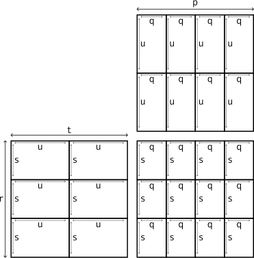
Fig. 10.7.1 Dimensions for the binary tensor contraction trus,pqtu->pqrs.

Fig. 10.7.1 illustrates the structure of the contraction for an instance with \(|r| = 3\), \(|t| = 2\), and \(|p| = 4\). Each tensor is drawn as a grid of tiles indexed by the schedule axes p, r, t, with each tile spanning the primitive axes s, q, u in its interior. Axis r aligns rows of tiles of in0 and out, axis p aligns columns of tiles of in1 and out, and axis t connects columns of tiles of in0 to rows of tiles of in1 through the contraction.

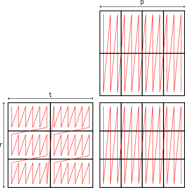
Fig. 10.7.2 Memory order for the binary tensor contraction trus,pqtu->pqrs.

Fig. 10.7.2 shows the memory order of the three tensors for the same instance. Within each tile, the unit-stride axes are s on in0 and out, and u on in1.

10.7.7. Parallel Tensor Contraction with BRGEMM

Building on Section 10.7.6, this example adds a second contraction axis to the Contraction primitive’s K role. With two K axes the lowering selects a BRGEMM kernel. Additionally, the example uses a schedule with two parallel iteration nodes.

Listing 10.7.13 Schedule tree for parallel BRGEMM-based tensor contraction trus,pqtu->pqrs.

p  (parallel)
└── r  (parallel)
    ├── zero
    └── brgemm

Listing 10.7.13 shows the schedule tree. The two iteration nodes p and r form the outer chain, both with policy parallel. Node r has two children, the invocation nodes zero and brgemm. The root list is roots = [p].

The axes are as in Table 10.7.15.

Table 10.7.22 Iteration nodes for parallel BRGEMM-based tensor contraction trus,pqtu->pqrs.

Node	Axis	Policy	Children	Guard
p	p	parallel	[r]	None
r	r	parallel	[zero, brgemm]	None

Table 10.7.23 Invocation nodes for parallel BRGEMM-based tensor contraction trus,pqtu->pqrs.

Node	Primitive	Guard
zero	zero_sq	None
brgemm	brgemm_sqtu	None

Table 10.7.22 lists the two iteration nodes, both with policy parallel. Node p has a single child, while node r has two children: the invocation nodes zero and brgemm. Table 10.7.23 specifies the two invocation nodes, neither of which carries a guard.

Table 10.7.24 TEIR-Primitives for parallel BRGEMM-based tensor contraction trus,pqtu->pqrs.

Primitive	Operation	Axes	Metadata
zero_sq	Zero	{M: [s], N: [q]}	{data_type: FP32}
brgemm_sqtu	Contraction	{M: [s], N: [q], K: [t, u]}	{data_type: FP32}

Table 10.7.24 defines the two primitives. zero_sq sets an \(|s| \times |q|\) output tile to zero in every invocation, while brgemm_sqtu accumulates into the same \(|s| \times |q|\) tile. M = [s], N = [q], and K = [t, u] make each brgemm_sqtu invocation a batch-reduce GEMM with two contraction axes.

Two new TEIR features combine here. First, a second axis in the K role of Contraction triggers BRGEMM lowering, with the outermost K axis as the batch-reduce dimension. Second, using the parallel iteration policy for nodes p and r allows the runtime to iterate these free axes in parallel.

Listing 10.7.14 Parallel BRGEMM-based execution of the tensor contraction trus,pqtu->pqrs.

#pragma omp parallel for collapse(2)
for p in 0 .. |p|-1
  for r in 0 .. |r|-1
     Zero( out = &out[p][0][r][0],
           ld  = |r|*|s| )
     Contraction( in0 = &in0[0][r][0][0],
                  in1 = &in1[p][0][0][0],
                  out = &out[p][0][r][0],
                  ldA     = |s|,
                  ldB     = |t|*|u|,
                  ldC     = |r|*|s|,
                  brSize  = |t|,
                  brStrA  = |r|*|u|*|s|,
                  brStrB  = |u| )

Lowering the configuration to nested loops produces the pseudocode in Listing 10.7.14. The parallel policy on both iteration nodes p and r lets the lowering parallelize the outer two loops. Here, this is illustrated by the OpenMP directive. Each (p, r) iteration first zeros its \(|s| \times |q|\) output tile and then invokes a single BRGEMM, which reduces over the two K axes t and u inside the primitive. Because distinct (p, r) iterations write disjoint output tiles, the per-iteration Zero and Contraction invocations are race-free under the parallel policy.